Using Amazon Machine Learning to Predict the Weather

Amazon recently launched their Machine Learning service, so I thought I’d take it for a spin. Machine Learning (ML) is all about predicting future data based on patterns in existing data. As an experiment I wanted to see if machine learning would be able to predict the weather of tomorrow based on weather observations. Weather systems travel large distances on a time scale of hours and days, so recent weather observations from around the country can be used to predict the future weather of one specific site. Meteorological institutes do this every day by running complex weather models on hundreds of nodes in large HPC clusters. I don’t expect machine learning to produce quite as good results as those models do, but thought it would be fun to see how close ML could get.

]

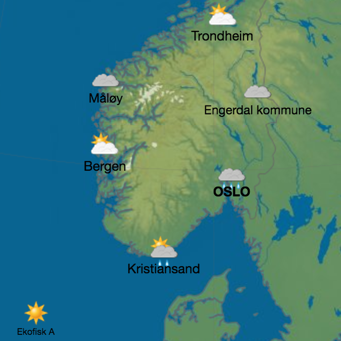Weather forecast from yr.no, delivered by the Norwegian Meteorological Institute and the NRK

The Amazon Machine Learning service makes it easy to get started and reduces the time it takes to get actionable insights from data. The service comes with tutorials, developer guides, a very useful explanation of machine learning concepts and enough tips to guide anyone through their first steps in the world of machine learning. There is a sample dataset you can use to create your first prediction model but if you want, you can follow along my journey in this post with my dataset instead. The source code to generate it is on Github and all you need to generate CSV files with weather observations is a free API key from Wunderground.com.

Defining the use case and dataset

Before diving into coding and machine learning, it’s important to define the use case as clearly as possible. To test whether Machine Learning is a viable approach to weather forecasting is the overall goal. To test this, I choose to predict the temperature tomorrow at 12:00 UTC in Oslo, the capital of Norway. The dataset I’ve chosen is weather observations from five cities in Norway, scattered around the southern half of the country. The weather in Oslo usually comes from the west, so I include observations from cities like Stavanger and Bergen in the dataset.

The layout of the dataset is important. Amazon Machine Learning treats every line in the dataset (CSV file) as a separate record and processes them randomly. For each record, it tries to predict the target value (temperature in Oslo the next day) from the variables present in that record. This means that you can’t rely on any connections between records, for example that the temperature measured at 10 AM may be similar to the temperature at 11 AM.

To create a dataset with enough data in each record to be able to predict the target value, I append all weather observations with the same timestamp, regardless of location, to the same record. This means that for any given timestamp there will for instance be five temperatures, five wind measurements and so on. To be able to distinguish between different cities in the dataset I named each column (each variable) with the first letter of the city name, forming variable names like “o_tempm” when the original observational data had a variable “tempm” containing the temperature for Oslo.

Creating the training dataset

Machine Learning works by creating a model from a training dataset where the target value to predict is already known. Since I want to predict a numerical value, Amazon ML defaults to a linear regression model. That is, it tries to build a formula which can output the target value, using individual weights for each variable in a record that tells the model how that variable is related to the target value. Some variables get weight zero, meaning they are not related to the target value at all, and others get positive weights between 0 and 1. To be able to determine weights for variables, there must be a sufficient amount of training data.

To create a sufficiently large training dataset, I needed weather observations for some time, at least 14 days. Fortunately, Wunderground.com has a JSON API that is really easy to use, and their history endpoint can provide weather observations for both the current date and dates back in time. I use that to collect observations for the last two weeks for all five cities. Since the free tier of their API restricts the use to 500 calls a day and maximum of 10 calls per minute, the script I made to generate the dataset has to wait some seconds between each API call. To limit the API usage and be able to rerun the script I cache weather observations on disk, because I don’t expect past weather observations to change.

A weather observation returned by their API has the following syntax:

{
  'conds': 'Light Rain Showers',
  'date': {
    'hour': '14',
    'mday': '29',
    'min': '00',
    'mon': '05',
    'pretty': '2:00 PM CEST on May 29, 2015',
    'tzname': 'Europe/Oslo',
    'year': '2015'
  },
  'dewpti': '35',
  'dewptm': '2',
  'fog': '0',
  'hail': '0',
  'heatindexi': '-9999',
  'heatindexm': '-9999',
  'hum': '36',
  'icon': 'rain',
  'metar': 'AAXX 29121 01384 11786 52108 10121 20015 51007 60001 78082 84260',
  'precipi': '',
  'precipm': '',
  'pressurei': '',
  'pressurem': '',
  'rain': '1',
  'snow': '0',
  'tempi': '54',
  'tempm': '12',
  'thunder': '0',
  'tornado': '0',
  'utcdate': {
    'hour': '12',
    'mday': '29',
    'min': '00',
    'mon': '05',
    'pretty': '12:00 PM GMT on May 29, 2015',
    'tzname': 'UTC',
    'year': '2015'
  },
  'visi': '37',
  'vism': '60',
  'wdird': '210',
  'wdire': 'SSW',
  'wgusti': '',
  'wgustm': '',
  'windchilli': '-999',
  'windchillm': '-999',
  'wspdi': '17.9',
  'wspdm': '28.8'
}

As you can see, this is the observation for May 29th at 12:00 UTC and the temperature was 12 degrees Celsius (“tempm”, where m stands for the metric system). The API returns a list of observations for a given place and date. The list contains observation data for at least every hour, some places even three times per hour. For each date and time, I combine the observations from all five places into one long record. If there isn’t data from all five places for that timestamp, I skip it, to make sure that all machine learning records have a sufficient amount of data. Lastly, for all records belonging to the training set, I append the target value (the next day’s temperature) as the last field. That way, I get a file “dataset.csv” with known target values that can be used to train the model. Here is an example record with the last number (8) being the target to predict:

20150515-22:00,,0,0,0,,56,,,0,0,6,0,0,10,180,South,,,7.2,Clear,3,0,0,,64,,1015,0,0,7,0,0,35,220,SW,,,10.8,,5,0,0,,76,,1014,0,0,8,0,0,,190,South,,,10.8,Clear,3,0,0,,68,,1013,0,0,7,0,0,30,190,South,,,18.0,Clear,-1,0,0,,66,,1013,0,0,3,0,0,45,130,SE,,,14.4,8

This way, I get a dataset where each timestamp is a separate record and all timestamps belonging to one date gets the next day’s temperature in Oslo at 12 UTC as the target value. In total 844 records for 14 days of observations.

In addition, the script outputs a file “testset.csv” with the last day of observations where the target value is unknown and should be predicted by the model.

Upload both CSV files to Amazon S3 before continuing, as Amazon Machine Learning is only able to use input data from S3 (or Redshift, but in that case Amazon exports it to S3 before using it). Be sure to select the “US Standard” region of S3, as the Machine Learning service is only available in their North Virginia location at the moment. To reduce costs it is important that the S3 datasets are in the same region as the Machine Learning service.

Create Amazon Machine Learning datasources

The datasource is an object used by the Machine Learning model to access the data in S3. Datasource objects contain a schema that tells the model what type of field each variable is (numeric, binary, categorical, text). This schema is autodetected when you create a datasource, but may need some review before continuing to make sure all field types were classified correctly.

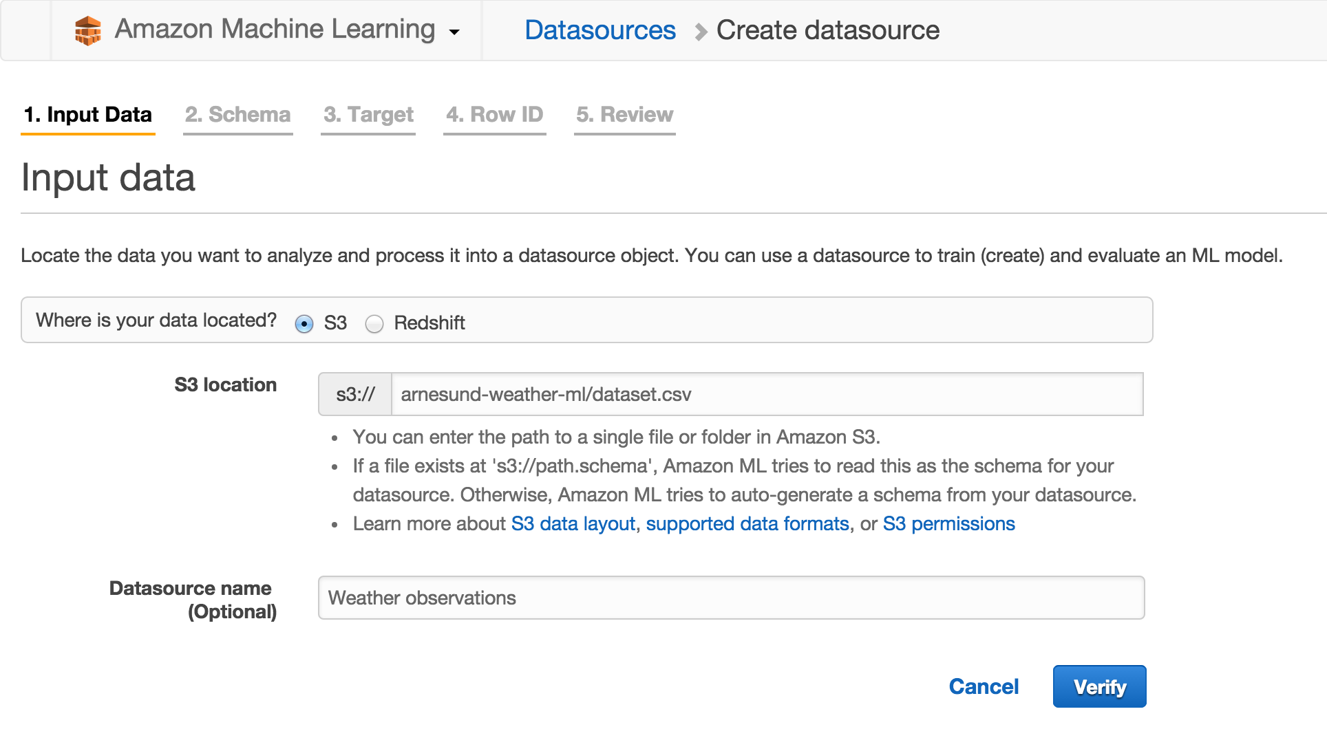
To create a datasource, first log into AWS to get access to Amazon Machine Learning. Select Create New -> Datasource. You are then asked for the path to the dataset in S3 and to give it a name, for instance “Weather observations”:

The dataset is verified and the schema is auto-generated. The next step is to make any adjustments to the schema if needed. Remember to say Yes to “Does the first line in your CSV contain the column names?”. I found that most fields containing actual data were correctly categorized, but fields with little or no data were not. There are some observation fields, like for instance “tornado”, that are normally zero for all five places and all times in my dataset. That field is binary but often autodetected as numeric (probably not an issue, since the field has no relevant data). The field “precipm” is numeric, but as it’s often blank (no precipitation detected) it can be mislabeled as categorical. Remember to go through all variables to check for misdetections like these, in my dataset there is 97 variables to check.

The third step is to define a target, which is the variable “target_o_tempm” in my dataset. When selected, Amazon Machine Learning informs you that “ML models trained from this datasource will use Numerical regression.” The last step in datasource creation is to define what field will be used as row identifier, in this case “datetime_utc”. The row identifier will be used to label output from the machine learning model, so it’s handy to use a value that’s unique to each record. The field selected as row identifier will be classified as Categorical. Review the settings and click Finish. It may take some minutes for the datasource to get status Completed, since Amazon does quite a bit of data analysis in the background. For each variable, the range of values is detected and scores like mean and median are computed.

At this point, I suggest you go ahead and create another datasource for the testset while you wait. The testset needs to have the same schema as the dataset used to train the model, which means that every field must have the same classification in both datasources. Therefore it’s smart to create the testset datasource right away when you still remember how each variable should be classified.

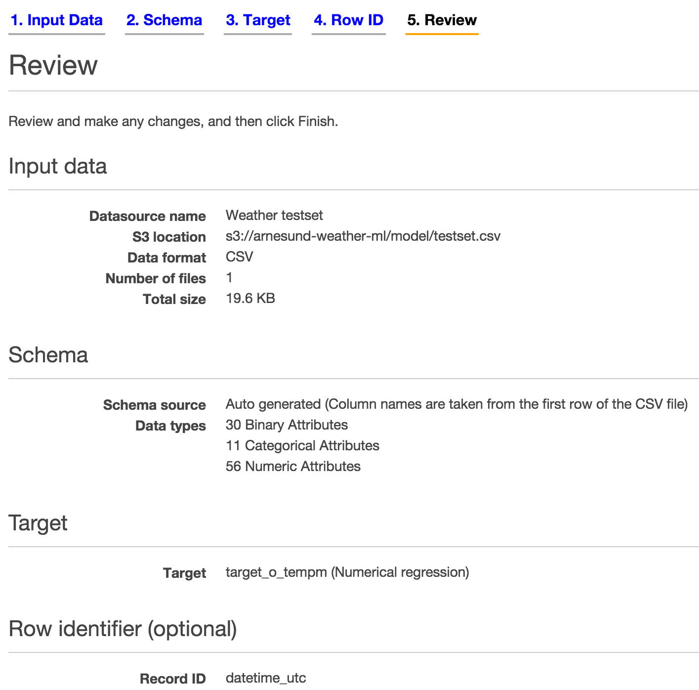
In my case I got 30 binary attributes (variables), 11 categorical attributes and 56 numeric attributes. The review page for datasource creation lists that information. Make sure the numbers match for the dataset and testset:

Creating the Machine Learning model

So, now you’ve got two datasources and can initialize model training. Most of the hard work in creating a dataset and the necessary datasources is already done at this point, so it’s time to put all this data to work and initialize creation of the model that is going to generate predictions.

Select Create New -> ML Model on the Machine Learning Dashboard page. The first step is to select the datasource you created for the dataset (use the “I already created a datasource pointing to my S3 data” option). The second step is the model settings, where the defaults are just fine for our use. Amazon splits the training dataset into two parts (a 70-30 split) to be able to both train the model and evaluate its performance. Evaluation is done using the last 30% of the dataset. The last step is to review the settings, and again, the defaults are fine. The advanced settings include options like how many passes ML should do over the dataset (default 10) and how it should do regularization. More on that below, just click Finish now to create the model. This will again take some time, as Amazon performs a lot of computations behind the scenes to train the model and evaluate its performance.

Regularization is a technique used to avoid overfitting of the model to the training dataset. Machine learning models are prone to both underfitting and overfitting problems. Underfitting means the model has failed at capturing the relation between input variables and target variable, so it is poor at predicting the target value. Overfitting also gives poor predictions and is a state where the model follows the training dataset too closely. The model remembers the training data instead of capturing the generic relations between variables. If for instance the target value in the training data fluctuates back and forth, the model output also fluctuates in the same manner. The result is errors and noise in the model output. When used on real data where the target value is unknown, the model will not be able to predict the value in a consistent way. This image helps explain the issue in a beautiful way:

Underfitting vs overfitting a machine learning model. Image source: http://knewt.ly/1dDB111

So to avoid overfitting, regularization is used. Regularization can be performed in multiple ways. Common techniques involve penalizing extreme variable weights and setting small weights to zero, to make the model less dependent on the training data and better at predicting unknown target values.

Exploring model performance

Remember that Amazon did an automatic split of the training data, using 70% of the records to train the model and the remaining 30% to evaluate the model. The Machine Learning service computes a couple of interesting performance metrics to inspect. Go to the Dashboard page and select the evaluation in the list of objects. The first metric shown is the RMSE, Root Mean Square Error, of the evaluation training data. The RMSE should be as low as possible, meaning the mean error is small and the predicted output is close to the actual target value. Amazon computes a baseline RMSE based from the model training data and compares the RMSE of the evaluation training data to that. In my testing I archieved an RMSE of about 2.5 in my first tests and near 2.0 after refining the dataset a bit. The biggest optimization I did was to change the value of invalid weather observations from the default value of -999 or -9999 to be empty. That way the range of values for each field got more close to the truth and did not include those very low numbers.

By selecting “Explore model performance”, you get access to an histogram showing the residuals of the model. Residuals are differences between predicted target and actual value. Here’s the plot for my model:

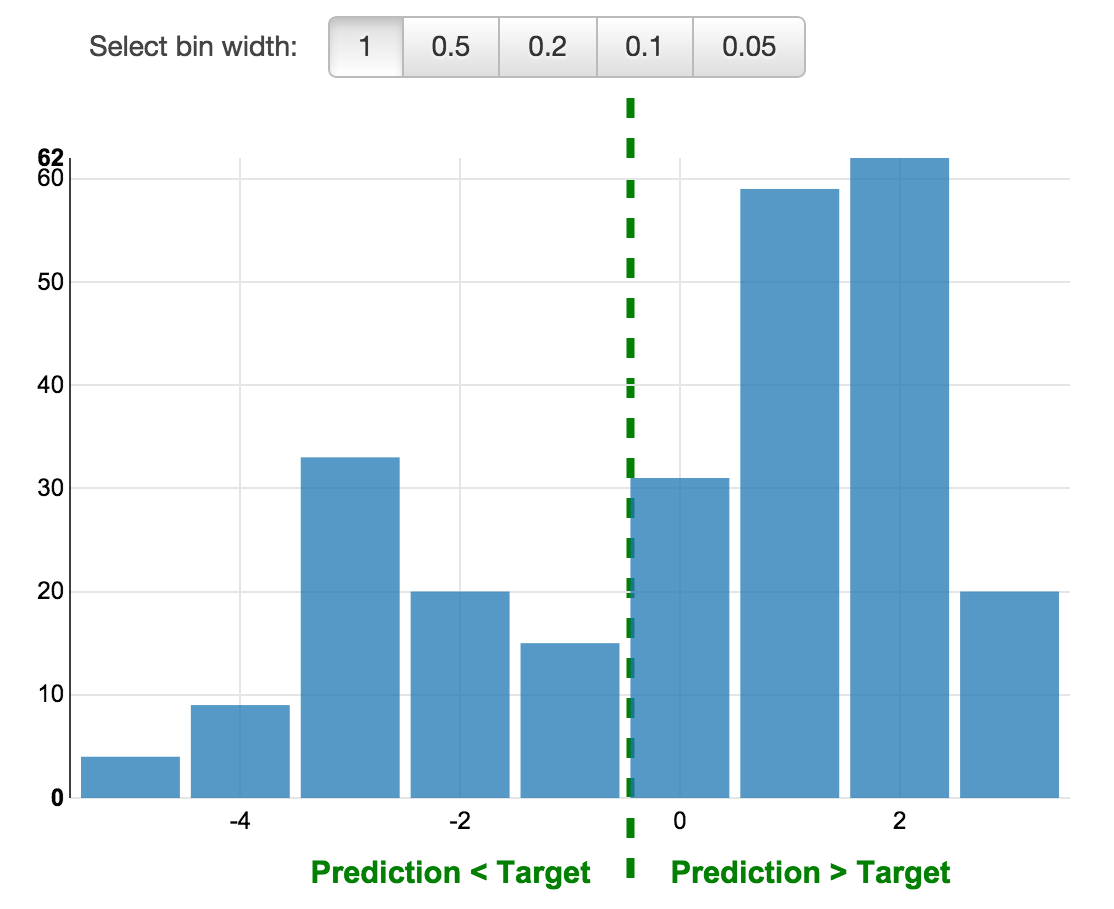Distribution of residuals

The histogram tells us that my model has a tendency to over-predict the temperature, and that a residual of 1 to 2 degrees Celcius is the most likely outcome. This is called a positive bias. To lower the bias it is possible to re-train the ML model with more data.

Before we use the model to predict temperatures, I’d like to show some of the interesting parts of the results of model training. Click the datasource for the training dataset on the Dashboard page to load the Data Report. Select Categorical under Attributes in the left menu. Sort the table by “Correlations to target” by clicking on that column. You’ll get a view that looks like this:

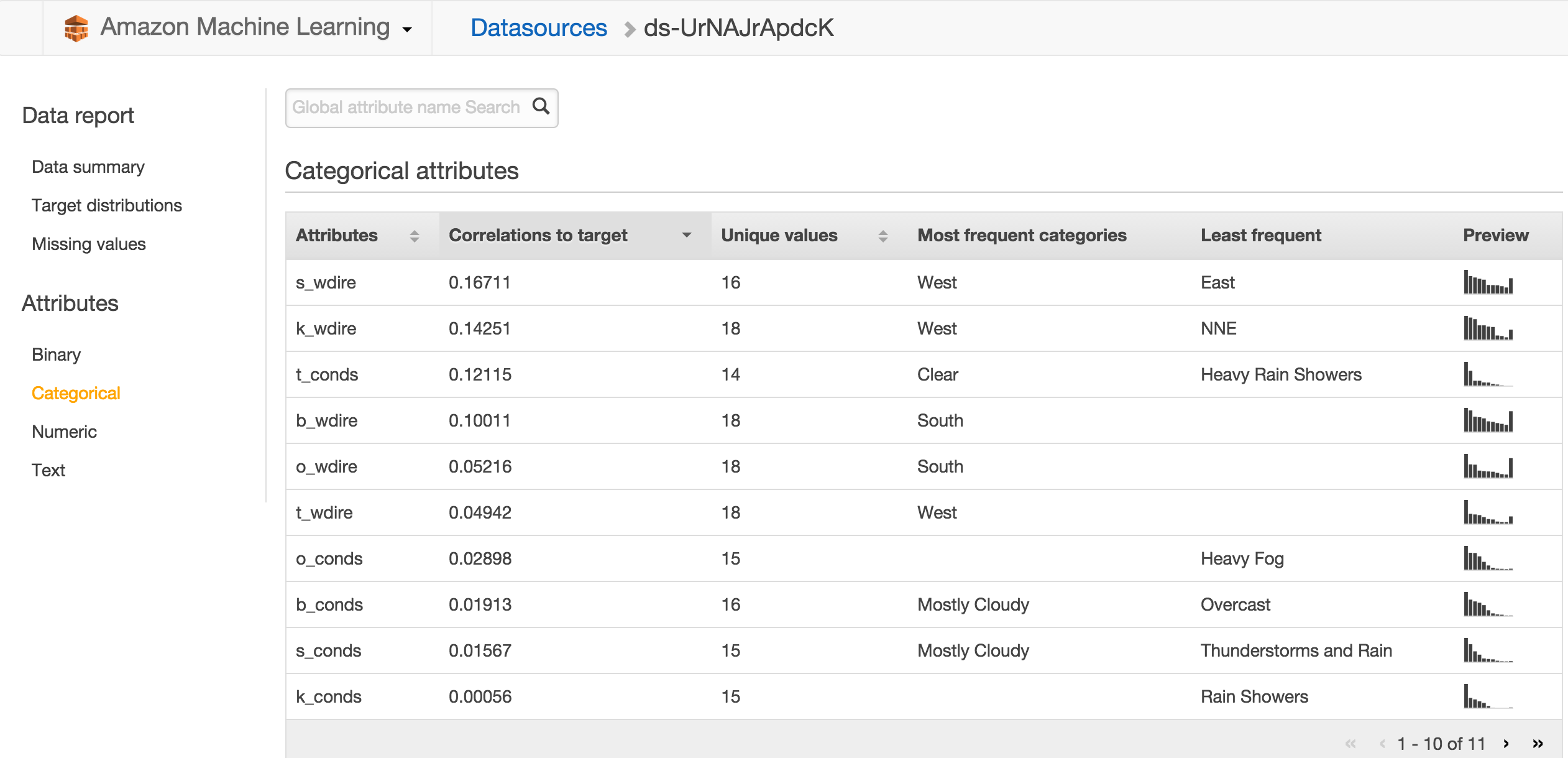
This table tells you how much weight each field has in determining the target value, so it is a good source of information on what the most important weather observation data are. Of the categorical attributes, the wind direction in Stavanger is the most important attribute for how the temperature is going to be in Oslo the next day. That makes sense since Stavanger is west of Oslo, so weather that hits Stavanger first is likely to arrive to Oslo later. Wind direction in Kristiansand is also important and in third place on this ranking we find the conditions in Trondheim. The most commonly observed values is shown along with a small view of the distribution for each variable. Click Numeric to see a similar ranking for those variables, revealing that dew point temperature for Trondheim and atmospheric pressure in Stavanger are the two most important numeric variables. For numeric variables, the range and mean of observed values is shown. It’s interesting to see that none of the mentioned important variables are weather observations from Oslo.

Use the model to predict the weather

The last step is to actually use the Amazon Machine Learning service to predict tomorrow’s temperature, by feeding the testset to the model. The testset contains one day of observations and an empty target value field.

Go back to the Dashboard and select the model in the object list. Click “Generate batch predictions” at the bottom of the model info page. The first step is to locate the testset datasource, which you’ve already created. When you click Verify Amazon checks that the schema of the testset matches the training dataset, which it should given that all variables have the same classification in both datasources. It is possible to create the testset datasource in this step instead of choosing an existing datasource. However, when I tried that, the schema of the testset was auto-generated with no option for customizing field classifications, so therefore it failed verification since the schema didn’t match the training dataset. That’s why I recommended you create a datasource for the testset too, not just for the training dataset.

After selecting the testset datasource, the last step in the wizard before review is choice of output S3 location. Amazon Machine Learning will create a subfolder in the location you supply. Review and Finish to launch the prediction process. Just like some of the previous steps, this may take some minutes to finish.

The results from the prediction process is saved to S3 as a gzip file. To see the results you need to locate the file in the S3 Console, download it and unpack it. The unpacked file is a CSV file, but lacks the “.csv” suffix, so you might need to add that to get the OS to recognize it properly. Results look like this:

tag,trueLabel,score
20150530-00:00,,1.503819E1
20150530-00:50,,1.342798E1
20150530-01:00,,1.297405E1
20150530-01:50,,1.321695E1
20150530-02:00,,1.270639E1
20150530-02:50,,1.271092E1
20150530-03:00,,1.309844E1
20150530-03:50,,1.444643E1
20150530-04:00,,1.373403E1

The “score” field is the predicted value, in this case the predicted temperature in Celsius. The tag reveals what observations resulted in the prediction, so for instance the observations from the five places for timestamp 02:00 resulted in a predicted temperature in Oslo the next day at 12:00 UTC of 12.7 degrees Celsius.

As you might have noticed, we’ve now got a bunch of predictions for the same temperature, not just one prediction. The strength in that is that we can inspect the distribution of predicted values and even how the predicted value changes according to observation timestamp (for example to check if weather observations from daytime give better predictions than those from the night).

Distribution of predicted temperature values

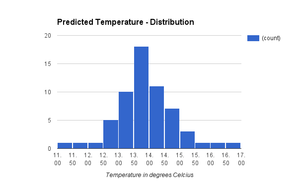
Even though the individual predictions differ, there seems to be strong indications that the value is between 13.0 and 14.5 degrees Celsius. Computing the mean over all predicted temperatures gives 13.6 degrees Celsius.

Development of predicted temperature values

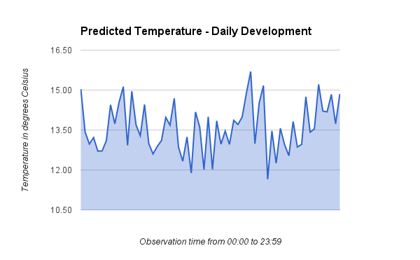
This plot shows the development in the predicted value as the observation time progresses. There does not seem to be any significant trend in how the different observation times perform.

The actual temperature - and some closing remarks

At this point I’m sure you wonder what the real temperature value ended up being. The value I tried to predict using Amazon Machine Learning turned out to be:

12:00 UTC on May 31, 2015:  12 degrees Celsius

Taking into account the positive bias of 1 to 2 degrees and a prediction mean value of 13.6 degrees Celsius, I am very satisfied with these results.

To improve the model performance further I could try to reduce the bias. To do that I’d have to re-train the model with more training data, since two weeks of data isn’t much. To get a model which could be used all year around, I’d have to include training data from a relevant subset of days throughout the year (cold days, snowy days, heavy rain, hot summer days and so on). Another possible optimization is to include more places in the dataset. The dataset lacks places to the east of Oslo, which is an obvious flaw. In addition to more data, I could explore if the dataset might need to be organized differently. It is for instance possible to append all observations from an entire day into one record, instead of creating a separate record for each observation timestamp. That would give the model more variables to use for prediction but then only one record to predict the value from.

It has been very interesting to get started with Amazon Machine Learning and test it with a real-life dataset. The power of the tool combined with the ease of use that Amazon has built into the service makes it a great offering. I’m sure I’ll use the service for new experiments in the future!