Using Facebook Prophet Forecasting Library to Predict the Weather

Facebook recently released a forecasting library for Python and R, called Prophet. It’s designed for forecasting future values of time series of any kind, and is remarkably easy to get started with. One of my favorite data sets are temperature time series, so here I’ll explore how good Prophet is at predicting future temperatures based on past weather observations.

The dataset consists of temperature readings every 10 minutes from my Netatmo Weather Station, stored in InfluxDB over at GrafAtmo.com. I extracted the mean temperature per hour for the last year, resulting in approx. 9000 hourly temperature observations.The timestamps are in ISO8601 format: “2016-02-11T08:00:00Z”. The dataset also has gaps due to several shorter periods of malfunctioning data collection and system maintenance. Prophet claims to handle such gaps without issues, so let’s see if it does.

If you want to try this out yourself, here’s the dataset!

Installing Prophet on Ubuntu Linux

Installing Prophet for Python is done using pip. Since Prophet depends on the Stan statistical library and is optimized for speed using C, it needs Cython and PyStan. In addition it depends on NumPy and Pandas, so make sure you have those installed too.

$ sudo -H pip install cython pystan numpy pandas
$ sudo -H pip install fbprophet

These can also be installed without sudo if you don’t have administrative privileges on the system.

Producing the first temperature predictions

To produce the initial predictions, we simply run through the following steps without changing default parameters.

Import packages and prepare input data

import pandas as pd
import numpy as np
from fbprophet import Prophet

df = pd.read_csv('outdoor-temperature-hourly.csv')
df = df[df.temperature != 'DIFF']

Preparing the dataset consists of loading it as a DataFrame using Pandas. The input dataset is a merge of two time series and some of the values are invalid. They are filtered out by excluding all rows with the value DIFF.

df['ds'] = df['time']
df['y'] = df['temperature']
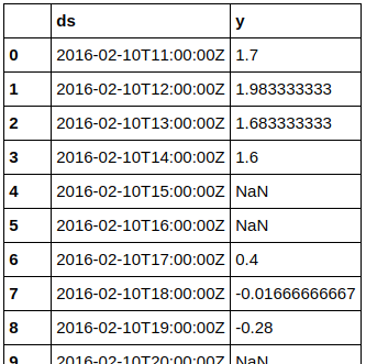
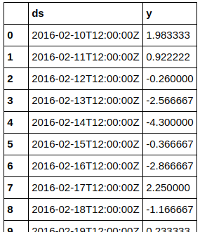
df = df.drop(['name', 'time', 'temperature', 'seriesA', 'seriesB'], axis=1)

Prophet requires one column named “ds” with dates or datetimes, and one column named “y” with numeric values. All other columns are ignored. The two required columns are created by duplicating two existing columns “time” and “temperature”, before all irrelevant columns are dropped from the dataframe. The preview shows the resulting dataframe which is used as input to Prophet. The values are degrees Celcius and timestamps are UTC. The input looks like this:

Fit model and use it to make predictions

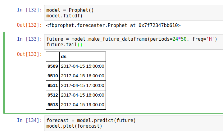
Fitting a model to the input data is as simple as “model.fit(df)”. To make predictions, you first need a DataFrame with datestamps to predict for. Prophet has a useful make_future_dataframe() method to do just that. By default it generates one row per day, but by setting the frequency parameter to “H” we get hours instead. In this example I generated a dataframe with 50 days of hourly timestamps, starting right after the most recent timestamp in the input dataset.

To make predictions based on the model, all you need to do is call “model.predict(future)”. Using the model and dataframe of future datetimes, Prophet predicts values for each future datetime.

Initial results

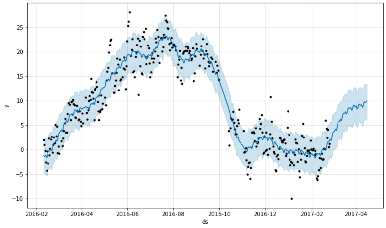
Prophet includes built-in plotting of the results using Matplotlib. Here’s the prediction for the hourly temperatures two months into the future, plotted as a continuation of the existing input data:

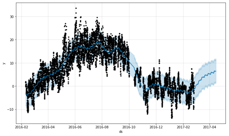
Pretty impressive output for so little work required! Prophet is fast too - these results were computed in only seconds. The temperature trends are clearly visible with higher hourly temperatures during the summer months than in the winter. The forecast for the next two months says that the temperatures are about to rise from around zero degrees Celcius currently to around 5 degrees in the start of April. However, the uncertainty intervals are quite large in this forecast (around 10 degrees). The somewhat large variations between day and night temperatures might cause this.

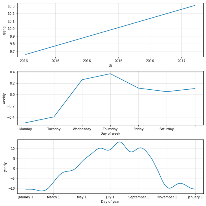
Before trying to reduce the uncertainty interval, let’s look at another output of the prediction model: The components of the model.

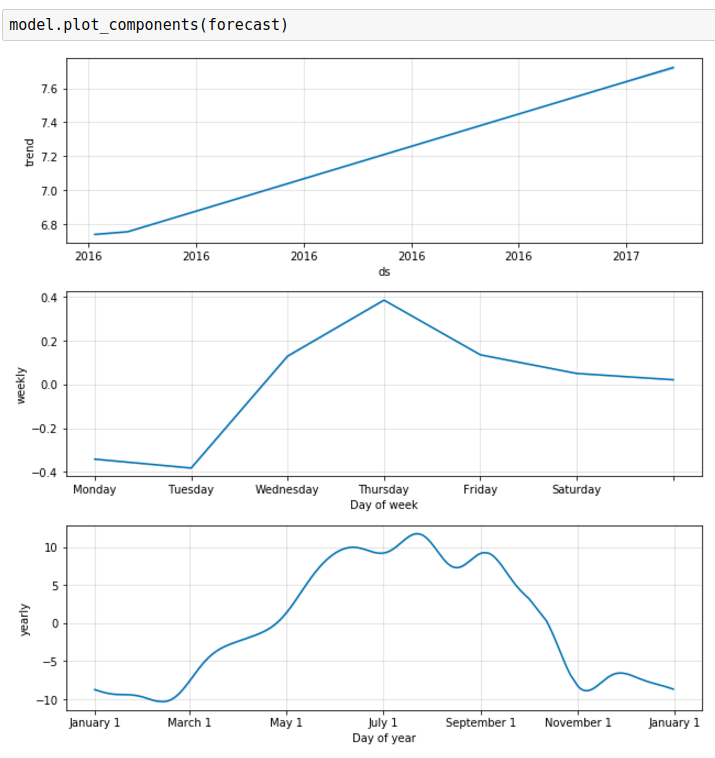
These subplots show several interesting patterns. The first subplot, “Trend” shows a slight temperature rise on the large scale, from year to year. As the input data only covers one year, this does not qualify as a generic trend. However, it does say that the recorded 2017-temperatures are slightly warmer than the 2016-temperatures.

The weekly trends are a bit strange. According to these results, the start of the week is colder than the rest of the week. As the weather doesn’t care about what day it is, this remains a curiosity.

The last plot shows the seasonal distribution of temperatures during the year of input data. Since I only had one year of input data, this plot follows the data as seen in the main plot pretty closely. Like in the trend subplot, the seasonal distributions would benefit from a lot more input data.

Tuning the model to only cover 2017

The initial results used the entire dataset, but how will Prophet behave if it doesn’t have input data from the same season last year to base the predictions on? Let’s investigate the results of using a smaller time period.

recent = df[df.ds > '2017-01-01']

Here I’m making a new input dataframe by selecting only the rows that have timestamps in 2017. Let’s make a new model and some new predictions too:

model_recent = Prophet()
model_recent.fit(recent)
future_recent = model_recent.make_future_dataframe(periods=24*10, freq='H')
forecast_recent = model_recent.predict(future_recent)

I set the period to make predictions for to 10 days into the future. Since the input data doesn’t cover nearly as much as in the initial results, it makes sense to reduce the number of days to predict for. The results are shown in the following graph.

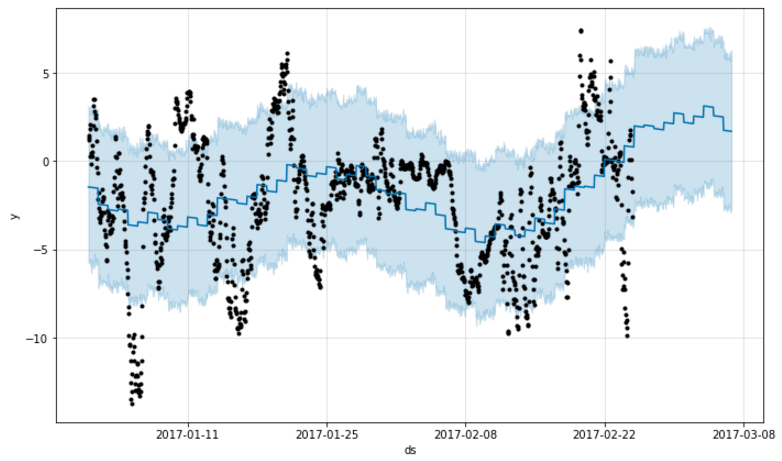
Since this plot covers a smaller time range, we can see more clearly the daily variations between day and night. Interestingly, Prophet is making the same type of prediction for the coming days as in the previous model; the temperature is going to rise. In this plot we can see why too. At around 2017-02-14 the temperature begun to rise and the last days of input data show temperatures well into the positive Celcius range. Prophet has successfully picked up this trend change and is using that to predict the future.

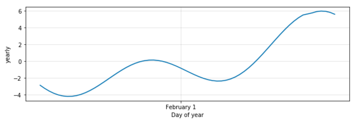
The Yearly trend subplot confirms that Prophet picked up on the trend change:

Tuning the model to reduce uncertainty intervals

In the initial results above, the uncertainty intervals were as big as 10 degrees Celcius. This is a bit too much to be useful in a weather forecasting system. To reduce the uncertainty, let’s make the input data a bit more uniform. To avoid having Prophet deal with day/night temperature differences, I filtered out all temperature measurements except for the one at 12:00 UTC each day. The theory is that these values, one per day, will be more uniform and lead to less variance in the model output.

Filtering the measurements could certainly be done using Pandas, but I chose to use the good old shell tools:

$ head -1 outdoor-temperature-hourly.csv > outdoor-temperature-12UTC.csv
$ fgrep "T12" outdoor-temperature-hourly.csv >> outdoor-temperature-12UTC.csv

Here I generate a new CSV file with only the temperature values for timestamps that contain “T12”. In the ISO8601 time format “T” is the date-time separator, so this selects all measurements having 12 as the hour component. I first save line 1 from the original file as line 1 in the new file to not lose column headings and having to tell Pandas about them manually.

Back in my Jupyter Notebook, the new input data is loaded into a dataframe like this:

df2 = pd.read_csv('outdoor-temperature-12UTC.csv', na_values = 'DIFF', usecols = ['time', 'temperature'])
df2['ds'] = df2['time']
df2['y'] = df2['temperature']
df2 = df2.drop('time', axis=1)
df2 = df2.drop('temperature', axis=1)

You might notice slight variations compared to the first example above. Here I added arguments to Pandas read_csv() to ignore lines with value DIFF and ignore all columns except the two with datetimes and values. Either way works, but I think this variant is a bit cleaner. To make sure we only got one temperature value per day, let’s have a look at the dataframe:

Looks good. By now you know the drill for making Prophet generate predictions:

model2 = Prophet()
model2.fit(df2)
future2 = model2.make_future_dataframe(periods=30)
forecast2 = model2.predict(future2)

The results

This is better. The uncertanty interval is down by approx. 30% to about 7 degrees. That means filtering the input data to one value per day increased the usefulness of the predictions, even though Prophet had less data to base predictions on.

The components of the model look similar to the first example:

Note that the first subplot, “Trend”, has higher values on the Y-axis than in the first example. That might be because I filtered out a lot of colder temperatures. 12 UTC is not the median temperature value during a typical day, it’s closer to the maximum (which is in the afternoon / early evening).

In addition to the subplots, we can inspect the predictions and components in depth by looking at the dataframe with predictions. The most interesting part is the timestamps in the future, so filter for them first:

import datetime
forecast2[forecast2.ds > datetime.datetime.now()]

This returns a dataframe with details about all predictions for all timestamps from now on. Here’s a screenshot of some of the contents (certain columns removed for brewity):

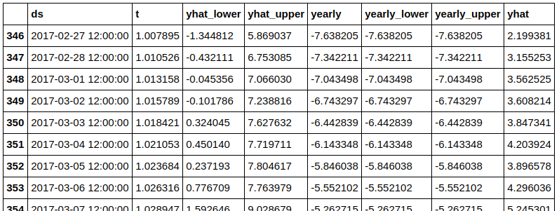
For each timestamp, you get the predicted value (“yhat”) in the rightmost column and all the components making up the prediction. For example we can see that the yearly components are well below zero degrees Celcius. This makes sense in the winter season. In addition, “yhat_lower” and “yhat_upper” show the exact range of the uncertainty interval.

Pro tip: Plot components with uncertainty intervals too

In the previous examples all the component subplots lack uncertainty intervals. Prophet can generate such intervals too, at the cost of longer computation time. This is done by adding a parameter to the model creation:

model2 = Prophet(mcmc_samples=500)

This gives you full Bayesian sampling and takes longer to complete, however it’s still just in the range of some minutes.

With this activated, we get component subplots with uncertainty intervals:

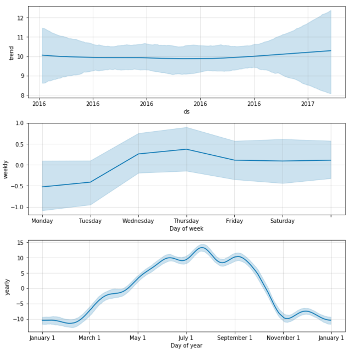
These plots reuse the filtered input data from the previous example, with one temperature value per day. We can now reconsider the strange weekly trend in the middle subplot, where the start of the week seems to be colder than the rest. The uncertainty is quite big in that plot. In addition the zero-degrees line is well within the uncertainty interval, for all days of the week. This means it’s not possible to say that there is any difference between the various weekdays.

Closing remarks

Using Prophet to generate predictions turned out to be very easy, and there are several ways to adjust the predictions and inspect the results. While there are other libraries that have more functionality and flexibility, Prophet hits the sweet spot of predictive power versus ease of use. No more looking at weird plots of predicted values because you chose the wrong algorithm for your use case. And no more spending hours to fix input data that has gaps or timestamps in the wrong format.

The Prophet forecasting library seems very well designed. It’s now my new favorite tool for ad-hoc trend analysis and forecasting!

~ Arne ~